Adaptive Component Separation with K-means Clustering

Learning Objectives

By the end of this notebook, you will:

• Understand adaptive sky clustering for spatially-varying spectral parameters

• Implement spherical K-means clustering for CMB component separation

• Optimize parameters within each cluster using variance-based selection

• Visualize how spatial parameter variation improves foreground modeling

The Adaptive Clustering Approach

Traditional component separation assumes uniform spectral parameters across the entire sky. In reality, Galactic emissions vary spatially. Our approach uses spherical K-means clustering to partition the sky into regions, allowing different spectral parameters in each cluster.

Key Innovation: Minimize CMB reconstruction variance by adaptively clustering sky pixels and optimizing spectral parameters per cluster.

!pip install -q furax-cs
!pip install --force-reinstall -r https://raw.githubusercontent.com/CMBSciPol/furax-cs/main/requirements.txt

# Setup and Data Loading


# Core libraries
# Data utilities
import operator
from functools import partial

import furax_cs as fcs
import healpy as hp

# JAX ecosystem
import jax
import jax.numpy as jnp
import matplotlib.pyplot as plt
import scienceplots  # noqa: F401

# FURAX framework
from furax.obs import negative_log_likelihood, sky_signal
from furax.obs.stokes import Stokes

# JAX-HEALPix for clustering and sky operations
from jax_healpy.clustering import (
    get_cutout_from_mask,
    get_fullmap_from_cutout,
)

# Configure JAX
jax.config.update("jax_enable_x64", True)

# Load CMB and foreground data
nside = 64
npixels = 12 * nside**2
noise_id = 0
noise_ratio = 1.0
tag = "c1d1s1"
mask_name = "ALL-GALACTIC"

# Generate and load multi-frequency data
fcs.save_to_cache(nside, sky=tag)
nu, freq_maps = fcs.load_from_cache(nside, sky=tag)
_, fg_maps = fcs.load_fg_map(nside, sky=tag)
cmb_map = fcs.load_cmb_map(nside, sky=tag)

print(f"Frequency maps shape: {freq_maps.shape}")
print(f"Frequencies: {len(nu)} bands from {nu[0]:.0f} to {nu[-1]:.0f} GHz")

# Convert to FURAX format (Q,U polarization)
d = Stokes.from_stokes(Q=freq_maps[:, 1, :], U=freq_maps[:, 2, :])
fg_stokes = Stokes.from_stokes(fg_maps[:, 1], fg_maps[:, 2])
cmb_map_stokes = Stokes.from_stokes(cmb_map[1], cmb_map[2])

# Load galactic mask (cleanest 20% of sky)
mask = fcs.get_mask(mask_name, nside=nside)
(indices,) = jnp.where(mask == 1)
coverage = jnp.mean(mask) * 100
print(f"Sky coverage: {coverage:.1f}% ({len(indices):,} pixels)")

# Extract masked data for computation
masked_d = get_cutout_from_mask(d, indices, axis=1)
masked_fg = get_cutout_from_mask(fg_stokes, indices, axis=1)
masked_cmb = get_cutout_from_mask(cmb_map_stokes, indices)
print(f"Masked data shape: {masked_d.shape}")

[INFO] Loaded freq_maps for nside 64 from cache with noise_ratio 0.0.
[INFO] Loaded freq_maps for nside 64 from cache.
[INFO] Loaded freq_maps for nside 64 from cache.
[INFO] Loaded freq_maps for nside 64 from cache.
Frequency maps shape: (15, 3, 49152)
Frequencies: 15 bands from 40 to 402 GHz
Sky coverage: 59.0% (29,009 pixels)
Masked data shape: (15, 29009)

Step 2: Spherical K-means Clustering

K-means clustering partitions the sky into regions with similar properties. For CMB component separation, we cluster pixels to allow different spectral parameters in each region.

Why Spherical K-means?

• Sky pixels are distributed on a sphere, not a flat plane

• Standard K-means would distort distances near poles

• Spherical K-means uses angular distance (great-circle distance)

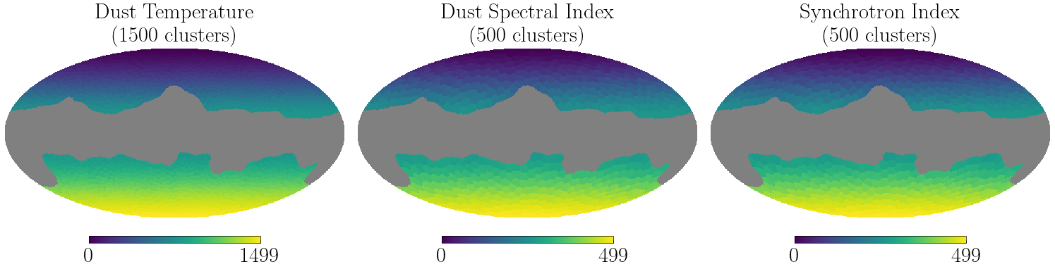
Cluster Configuration

Each spectral parameter can have a different number of clusters:

• Dust temperature: Varies slowly → fewer clusters needed

• Dust spectral index: More spatial variation → more clusters

• Synchrotron index: Varies slowly → fewer clusters

Step 3: Noise Model Setup

Real CMB observations contain instrumental noise. We model this as:

• White noise: Uncorrelated between pixels and frequencies

• Noise variance: Determined by instrument sensitivity

The noise covariance operator N is diagonal (independent noise per pixel/frequency).

Step 4: Parameter Optimization

We minimize the negative log-likelihood to find optimal spectral parameters for each cluster.

The Likelihood Function

The marginalized likelihood integrates over component amplitudes:

\[\mathcal{L}(\beta) = (A^T N^{-1} d)^T (A^T N^{-1} A)^{-1} (A^T N^{-1} d)\]

Optimization Strategy

• Solver: L-BFGS with zoom linesearch for fast convergence

• Bounds: Physical constraints on parameters (e.g., positive temperature)

• Analytical gradients: More stable than autodiff for this problem

Step 5: Parameter Map Reconstruction

After optimization, we map the per-cluster parameters back to the full sky:

1. Each pixel belongs to a cluster

2. The cluster’s optimized parameter value is assigned to all its pixels

3. Masked regions remain as UNSEEN

# Spherical K-means Clustering
# Configure clustering parameters for different spectral indices
cluster_config = {
    "temp_dust": 500,  # Dust temperature clusters
    "beta_dust": 1500,  # Dust spectral index clusters
    "beta_pl": 500,  # Synchrotron spectral index clusters
}
cluster_config = jax.tree.map(lambda x: min(indices.size, x), cluster_config)

# Generate clusters for each parameter type
print("Generating spherical K-means clusters...")
clusters = {}

# Generate spherical K-means clusters on unmasked pixels
masked_clusters = fcs.kmeans_clusters(
    jax.random.PRNGKey(42),  # Fixed seed for reproducibility
    mask,
    indices,
    cluster_config,
    initial_sample_size=1,
)

masked_clusters = {f"{param}_patches": patches for param, patches in masked_clusters.items()}

print("Clustering complete!")

Generating spherical K-means clusters...
Clustering complete!

full_mask_cluster = get_fullmap_from_cutout(masked_clusters, indices, nside=nside)

# Visualize the clustering results
fig = plt.figure(figsize=(15, 5))

param_labels = ["Dust Temperature", "Dust Spectral Index", "Synchrotron Index"]
for i, (param, label) in enumerate(zip(cluster_config.keys(), param_labels)):
    cluster_data = full_mask_cluster[f"{param}_patches"]
    n_unique = jnp.unique(cluster_data[cluster_data != hp.UNSEEN]).size

    hp.mollview(
        cluster_data,
        title=f"{label}\n({n_unique} clusters)",
        sub=(1, 3, i + 1),
        bgcolor=(0.0,) * 4,
    )

plt.tight_layout()
plt.show()

/tmp/ipykernel_11677/3066409688.py:18: UserWarning: This figure includes Axes that are not compatible with tight_layout, so results might be incorrect.
  plt.tight_layout()

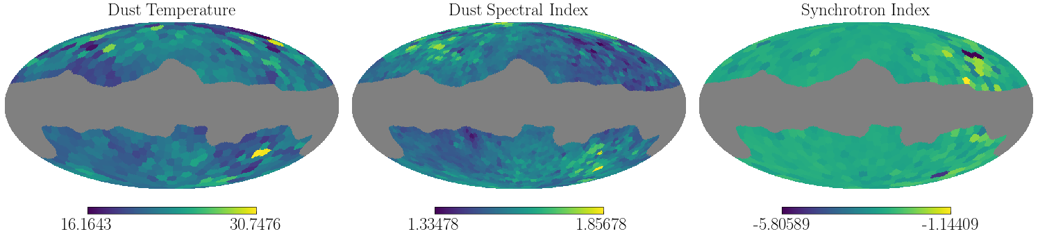
Step 6: Results Visualization

The recovered parameter maps show spatial variation in foreground properties:

• Dust temperature: ~20K in most regions

• Dust spectral index: ~1.5 with spatial variation

• Synchrotron index: ~-3.0 with gradients

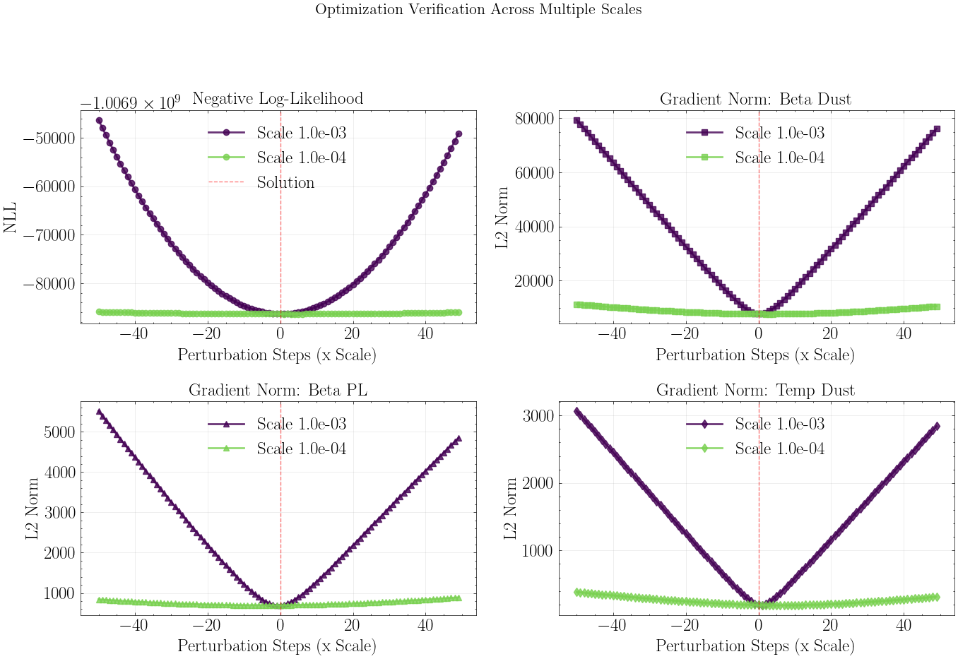
Step 7: Optimization Verification

To verify the optimizer found a true minimum, we perturb the solution and check:

1. NLL increases when moving away from the solution

2. Gradient norms are minimized at the solution

This confirms the optimization converged correctly.

noise_id = 0

instrument = fcs.get_instrument("LiteBIRD")
nu = instrument.frequency

key = jax.random.PRNGKey(noise_id)
noised_d, N, _ = fcs.generate_noise_operator(
    key, noise_ratio, indices, nside, masked_d, instrument, stokes_type="QU"
)
N.in_structure

StokesQU(q=ShapeDtypeStruct(shape=(15, 29009), dtype=float64), u=ShapeDtypeStruct(shape=(15, 29009), dtype=float64))

# Parameter Optimization

# Setup optimization parameters
dust_nu0 = 150.0  # Dust reference frequency (GHz)
synchrotron_nu0 = 20.0  # Synchrotron reference frequency (GHz)
SOLVER_BACKEND = "ADABK0"  # Options: "optax_lbfgs", "scipy_tnc", "active_set"
TOLERANCE = 1e-16
MAX_ITER = 2000

# Create objective function with fixed reference frequencies
negative_log_likelihood_fn = partial(
    negative_log_likelihood,
    dust_nu0=dust_nu0,
    synchrotron_nu0=synchrotron_nu0,
    analytical_gradient=True,
)

sky_signal_fn = partial(sky_signal, dust_nu0=dust_nu0, synchrotron_nu0=synchrotron_nu0)

# Initialize parameters for each cluster (realistic starting values)
initial_params = {
    "temp_dust": jnp.full((cluster_config["temp_dust"],), 20.0),  # 20K dust temperature
    "beta_dust": jnp.full((cluster_config["beta_dust"],), 1.54),  # Dust spectral index
    "beta_pl": jnp.full((cluster_config["beta_pl"],), -3.0),  # Synchrotron index
}
lower_bound = {
    "beta_dust": 0.5,
    "temp_dust": 10.0,
    "beta_pl": -7.0,
}
upper_bound = {
    "beta_dust": 3.0,
    "temp_dust": 40.0,
    "beta_pl": -0.5,
}

print("Parameter initialization:")
for param, values in initial_params.items():
    print(f"  {param}: {len(values)} clusters, initial value = {values[0]}")

print("\nRunning optimization...")
print(f"Using solver: {SOLVER_BACKEND}")
print("This may take a few minutes...")

# Run optimization using unified minimize API
final_params, final_state = fcs.minimize(
    fn=negative_log_likelihood_fn,
    init_params=initial_params,
    solver_name=SOLVER_BACKEND,
    max_iter=MAX_ITER,
    rtol=TOLERANCE,
    atol=TOLERANCE,
    lower_bound=lower_bound,
    upper_bound=upper_bound,
    nu=nu,
    N=N,
    d=noised_d,
    patch_indices=masked_clusters,
)

Parameter initialization:
  temp_dust: 500 clusters, initial value = 20.0
  beta_dust: 1500 clusters, initial value = 1.54
  beta_pl: 500 clusters, initial value = -3.0

Running optimization...
Using solver: ADABK0
This may take a few minutes...
[INFO] key active_set: max_constraints_to_release=1 / 2500 params

100.00%|██████████| [18:39<00:00, 11.20s/%]

The Kernel crashed while executing code in the current cell or a previous cell.

Please review the code in the cell(s) to identify a possible cause of the failure.

Click <a href='https://aka.ms/vscodeJupyterKernelCrash'>here</a> for more info.

View Jupyter <a href='command:jupyter.viewOutput'>log</a> for further details.

# Show optimization results
print("\nOptimization completed!")
print(f"Final function value: {final_state.best_loss:.2e}")

# Display optimized parameter statistics
print("\nOptimized parameter ranges:")
for param, values in final_params.items():
    print(
        f"  {param}: [{jnp.min(values):.3f}, {jnp.max(values):.3f}], "
        f"mean = {jnp.mean(values):.3f} ± {jnp.std(values):.3f}"
    )

# Compute CMB reconstruction with optimized parameters
reconstructed_signal = sky_signal_fn(
    final_params, nu=nu, d=masked_d, N=N, patch_indices=masked_clusters
)
nll = negative_log_likelihood_fn(
    final_params, nu=nu, d=noised_d, N=N, patch_indices=masked_clusters
)

cmb_reconstruction = reconstructed_signal["cmb"]
cmb_var = jax.tree.reduce(operator.add, jax.tree.map(jnp.var, cmb_reconstruction))
cmb_np = jnp.stack([cmb_reconstruction.q, cmb_reconstruction.u])
print("\nCMB reconstruction completed")
print(f"CMB shape: Q={cmb_reconstruction.q.shape}, U={cmb_reconstruction.u.shape}")

Optimization completed!
Final function value: -1.01e+09

Optimized parameter ranges:
  beta_dust: [1.335, 1.857], mean = 1.537 ± 0.061
  beta_pl: [-5.806, -1.144], mean = -2.966 ± 0.330
  temp_dust: [16.164, 30.748], mean = 21.764 ± 1.771

CMB reconstruction completed
CMB shape: Q=(29009,), U=(29009,)

# Parameter Map Reconstruction

# Map cluster parameters back to full sky maps
print("Reconstructing full-sky parameter maps...")

param_maps = {}
for param_name in ["temp_dust", "beta_dust", "beta_pl"]:
    # Get optimized parameter values for each cluster
    param_values = final_params[param_name]
    cluster_indices = masked_clusters[f"{param_name}_patches"]

    # Map parameter values to masked pixels using cluster assignments
    param_map_masked = param_values[cluster_indices]

    # Convert back to full HEALPix map
    full_param_map = get_fullmap_from_cutout(param_map_masked, indices, nside=nside)
    param_maps[param_name] = full_param_map

print("Parameter map reconstruction completed!")

# Also reconstruct CMB maps for visualization
cmb_q_full = get_fullmap_from_cutout(cmb_reconstruction.q, indices, nside=nside)
cmb_u_full = get_fullmap_from_cutout(cmb_reconstruction.u, indices, nside=nside)

print("CMB maps reconstructed to full sky")
print(f"Parameter maps available: {list(param_maps.keys())}")

# Display parameter statistics
print("\\nFull-sky parameter statistics:")
for param_name, param_map in param_maps.items():
    valid_data = param_map[param_map != hp.UNSEEN]
    if len(valid_data) > 0:
        print(
            f"  {param_name}: [{jnp.min(valid_data):.3f}, {jnp.max(valid_data):.3f}], "
            f"mean = {jnp.mean(valid_data):.3f} ± {jnp.std(valid_data):.3f}"
        )
    else:
        print(f"  {param_name}: No valid data")

Reconstructing full-sky parameter maps...
Parameter map reconstruction completed!
CMB maps reconstructed to full sky
Parameter maps available: ['temp_dust', 'beta_dust', 'beta_pl']
\nFull-sky parameter statistics:
  temp_dust: [16.164, 30.748], mean = 21.735 ± 1.756
  beta_dust: [1.335, 1.857], mean = 1.538 ± 0.061
  beta_pl: [-5.806, -1.144], mean = -2.969 ± 0.321

# Results Visualization
fig = plt.figure(figsize=(15, 5))

# Plot the three parameter maps only
hp.mollview(param_maps["temp_dust"], title="Dust Temperature", sub=(1, 3, 1), bgcolor=(0.0,) * 4)

hp.mollview(param_maps["beta_dust"], title="Dust Spectral Index", sub=(1, 3, 2), bgcolor=(0.0,) * 4)

hp.mollview(param_maps["beta_pl"], title="Synchrotron Index", sub=(1, 3, 3), bgcolor=(0.0,) * 4)

plt.tight_layout()
plt.show()

/tmp/ipykernel_73191/1189568572.py:11: UserWarning: This figure includes Axes that are not compatible with tight_layout, so results might be incorrect.
  plt.tight_layout()

import jax
import jax.numpy as jnp
import matplotlib.pyplot as plt

# 1. Define Multiple Scales
scales = [1e-3, 1e-4]  # You can add more scales here
points = 100
steps = jnp.arange(-points // 2, points // 2)


# 2. Define JIT-compiled functions (compiled once)
@jax.jit
def grad_nll(params):
    return jax.grad(negative_log_likelihood_fn)(
        params,
        nu=nu,
        N=N,
        d=masked_d,
        patch_indices=masked_clusters,
    )


@jax.jit
def eval_nll(params):
    return negative_log_likelihood_fn(
        params,
        nu=nu,
        N=N,
        d=masked_d,
        patch_indices=masked_clusters,
    )


# 3. Setup Plotting Grid
fig, axes = plt.subplots(2, 2, figsize=(14, 10))
fig.suptitle("Optimization Verification Across Multiple Scales", fontsize=16)

# Colors for different scales
colors = plt.cm.viridis(jnp.linspace(0, 0.8, len(scales)))

print("Computing NLLs and Gradients for multiple scales...")

# 4. Loop over scales
for i, scale in enumerate(scales):
    print(f"  Processing scale: {scale:.1e}")

    # Calculate perturbations for this scale
    perturbations = steps.reshape(-1, 1) * scale

    # Perturb Parameters
    final_params_perturbed = jax.tree.map(lambda p: p.reshape(1, -1) + perturbations, final_params)

    # Compute Results
    nlls = jax.vmap(eval_nll)(final_params_perturbed)
    grads = jax.vmap(grad_nll)(final_params_perturbed)

    # Extract Norms
    grads_beta_dust_norm = jnp.linalg.norm(grads["beta_dust"], axis=1)
    grads_beta_pl_norm = jnp.linalg.norm(grads["beta_pl"], axis=1)
    grads_temp_dust_norm = jnp.linalg.norm(grads["temp_dust"], axis=1)

    # --- Plotting for this scale ---
    label = f"Scale {scale:.1e}"
    color = colors[i]

    # Plot 1: Negative Log Likelihood
    ax = axes[0, 0]
    ax.plot(steps, nlls, "o-", linewidth=2, color=color, label=label, alpha=0.8)

    # Plot 2: Gradient Norm - Beta Dust
    ax = axes[0, 1]
    ax.plot(steps, grads_beta_dust_norm, "s-", linewidth=2, color=color, label=label, alpha=0.8)

    # Plot 3: Gradient Norm - Beta PL
    ax = axes[1, 0]
    ax.plot(steps, grads_beta_pl_norm, "^-", linewidth=2, color=color, label=label, alpha=0.8)

    # Plot 4: Gradient Norm - Temp Dust
    ax = axes[1, 1]
    ax.plot(steps, grads_temp_dust_norm, "d-", linewidth=2, color=color, label=label, alpha=0.8)

# 5. Final Plot Formatting
# NLL Plot
ax = axes[0, 0]
ax.set_title("Negative Log-Likelihood")
ax.set_ylabel("NLL")
ax.set_xlabel("Perturbation Steps (x Scale)")
ax.grid(True, alpha=0.3)
ax.axvline(0, color="red", linestyle="--", alpha=0.5, label="Solution")
ax.legend()

# Beta Dust Grad Plot
ax = axes[0, 1]
ax.set_title("Gradient Norm: Beta Dust")
ax.set_ylabel("L2 Norm")
ax.set_xlabel("Perturbation Steps (x Scale)")
ax.grid(True, alpha=0.3)
ax.axvline(0, color="red", linestyle="--", alpha=0.5)
ax.legend()

# Beta PL Grad Plot
ax = axes[1, 0]
ax.set_title("Gradient Norm: Beta PL")
ax.set_ylabel("L2 Norm")
ax.set_xlabel("Perturbation Steps (x Scale)")
ax.grid(True, alpha=0.3)
ax.axvline(0, color="red", linestyle="--", alpha=0.5)
ax.legend()

# Temp Dust Grad Plot
ax = axes[1, 1]
ax.set_title("Gradient Norm: Temp Dust")
ax.set_ylabel("L2 Norm")
ax.set_xlabel("Perturbation Steps (x Scale)")
ax.grid(True, alpha=0.3)
ax.axvline(0, color="red", linestyle="--", alpha=0.5)
ax.legend()

plt.tight_layout(rect=[0, 0.03, 1, 0.95])
plt.show()

Computing NLLs and Gradients for multiple scales...
  Processing scale: 1.0e-03
  Processing scale: 1.0e-04